HELP
Structure of the MPM Online Tool
-
The
MPM online tool is a geographic information systems (GIS) modelling tool for
modelling of mineral prospectivity in northern
Finland.
-
The
MPM online tool is composed of GTK open source geospatial datasets and fuzzy
logic modelling tools.
-
The
input data i.e. raster layers and other GIS dataset helping to localize and
assess modelling results are located on the left hand side of the tool under
the 'Layers' (Fig. 1). 'Derivatives' are generated from the geological GIS data
such as distance to structures and density of structures. The airborne
geophysical data consists of magnetic and electromagnetic interpolated
measurement data. The geochemical data is interpolated from glacial till assay
data (see Data for specifications). Unfortunately, in the current version of
the MPM online tool the histogram stretching of the colour scale cannot be
performed by the user.
-
The
spatial representation of the input and output layers, and other exploration
related data layers, can be viewed in the 'Map' (Fig. 1).
-
Fuzzy
tools i.e. 'Fuzzy Membership' and 'Fuzzy Overlay' tools are located on the top
right corner of the MPM online tool (Fig. 1).
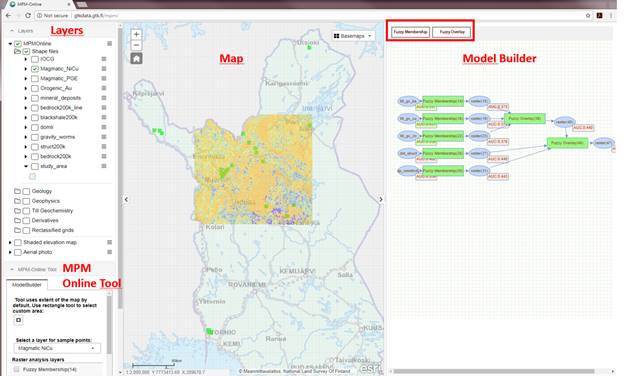
Fig. 1. The
user interphase of the Mineral Prospectivity Modeler Online Tool.
-
To
produce a prospectivity model, the input data and
fuzzy modelling tools are arranged into a geoprocessing
model to the 'Model Builder' located on the right hand side of the MPM online
tool (Fig. 2).
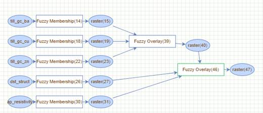
Figure 2. An example
-
'Bookmarks'
at the bottom left of the MPM online tool can help to zoom into a focus area.
Construction of a mineral prospect model in the
Model Builder
-
The
input data and fuzzy tools can be dragged with the left hand mouse button and
dropped one dataset or a tool at a time to the Model Builder (Fig. 2).
Copy-pasting of the data ellipses and tool rectangles is not possible in the
current version of the MPM tool.
-
A
raster input and output can be removed by clicking on to the raster ellipse
(outlines turn green) and pressing the delete button on the keyboard.
-
An
input raster dataset can be connected to a Fuzzy Membership tool by bringing
the cursor on top of an ellipse representing the input raster (see Fig. 3).
When the cursor turns into a hand icon click onto ellipse with the right mouse
button. Keep the right mouse button down and move the cursor onto the Fuzzy
Membership tool. Release the mouse button and the input raster layer and the
fuzzy tool should be connected with an arrow.
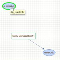
Figure 3. Connect an input layer (ap_resistivity) to the Fuzzy Membership tool by drawing an
arrow in the Model Builder. The output of the Fuzzy Membership,
in this example case, is raster(15).
-
For
the modelling result to be meaningful each input dataset has to be transformed
with Fuzzy Membership tool before Fuzzy Overlay. The fuzzy logic as an expert
driven machine learning technique is described in 'Fuzzy logic' and the details
of the fuzzy tools at http://desktop.arcgis.com/en/arcmap/10.3/tools/spatial-analyst-toolbox/an-overview-of-the-overlay-tools.htm
-
The
membership is always scaled between 0 and 1. Thus, if the real minimum
membership is more than 0 or the real maximum less than 1, the memberships have
to be transformed to the correct range using other tools which are not yet
available in the MPM Online Tool.
-
The
Fuzzy Membership tool parameters are shortly described in table 1. For more
detailed information go to
http://desktop.arcgis.com/en/arcmap/10.3/tools/spatial-analyst-toolbox/fuzzy-membership.htm
and click to see the specifications for each function.
|
Fuzzy membership
tool parameter |
Option |
Explanation |
|
Fuzzy
membership type |
Large |
The fuzzy
membership transformation function 'Large' defines the shape of the fuzzy
membership function as an S-shape increasing function. The small values of
input data will be close to 0 and large values close to 1. |
|
|
Gaussian |
Defines
the shape of the fuzzy membership function as an
Gaussian bell shaped function. The small and large values of input data will
be close to 0 and values close the mid point close
to 1. |
|
|
Near |
Near
function is similar to the Gaussian fuzzy membership function except the Near
function has a more narrow spread. |
|
|
Small |
Defines
the shape of the fuzzy membership function as an S-shape decreasing function.
The small values of input data will be close to 1 and large values close to
0. |
|
Mid point |
|
Defines
the value of the input data with a fuzzy membership of 0.5. The default value
of the mid point is mean of the dataset if the mid point field in the tool is left empty. The processing
extent is considered when the mean value is calculated. |
|
Spread |
|
Defines
the spread of a function. For the Large and Small functions the spread values
range from 1 to 10, for Gaussian from 0.01 to 1 and for Near from 0.001 to 1.
Larger values result in a steeper distribution from the midpoint. |
|
Hedge |
None |
Defining
a hedge increases or decreases the fuzzy membership values which modify the
meaning of a fuzzy set. Hedges are useful to help in controlling the criteria
or important attributes. NONE -No
hedge is applied. This is the default. |
|
|
Somewhat |
SOMEWHAT
'Known as dilation, defined as the square root of the fuzzy membership
function. This hedge increases the fuzzy membership functions. |
|
|
Very |
VERY
-Also known as concentration, defined as the fuzzy membership function
squared. This hedge decreases the fuzzy membership functions. |
Table 1. Parameters of the Fuzzy Membership
functions and their specifications.
-
To
specify the parameters a Fuzzy Membership tool can be opened by double clicking
the Fuzzy Membership rectangle. An additional window opens up to specify the
parameters (Fig. 4).
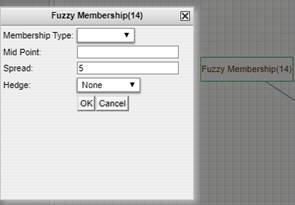
Figure 4. The Fuzzy Membership tool. Specify
the Fuzzy Membership type, Mid
point, Spread and Hedge.
- Determination
of the midpoint is critical for the success of the modelling. In the current
version of the MPM online tool, there is no tool to study the distribution of
the data e.g. as a histogram or descriptive statistics besides the mean. If the
midpoint field in the Fuzzy Membership tool is left empty the tool uses mean of
the input data as a mid point. In this case, the
chosen extent is considered. It is an advisable practice to run a Fuzzy
Membership tool first with an empty mid point field
and keep notes of the used mid point which is
reported in the 'Running model...'-window and updated back to tool if it was
originally left empty. This way the user
will know the mean value of the data and can then start to increase or decrease
it manually for the following runs of the model.
- Connect
the Fuzzy Membership output rasters to each other
with Fuzzy Overlay tool. The assumption is that the user has scaled the inputs
between 0 and 1 prior to combining them with a Fuzzy Overlay function.To specify the parameters the Fuzzy Membership
tool can be opened by double clicking the Fuzzy Overlay rectangle. An
additional window opens up to specify the parameters (Fig. 5).
-
The
Fuzzy Overlay types and their short definition is given in table 2.
-
To
view active parameters of the tool, hover the mouse over tool and the tooltip
opens.
|
Overlay
type |
|
|
AND |
Returns
the minimum value of all of the input evidence rasters
for each cell. |
|
OR |
Returns the
maximum value of all of the input evidence rasters
for each cell. |
|
SUM |
Calculates
the product of unfavourabilities of all the input rasters and subtracts this from unity for each cell.
Tends towards large values if even one of the inputs has a large value or if
many inputs have intermediate values. |
|
PRODUCT |
Calculates the product of values of all the
input rasters for each cell. Tends towards small
values, if even one of the inputs has a small value or if many inputs have
intermediate values. |
|
GAMMA |
The GAMMA
type is typically used to combine more basic data. When gamma is 1, the
result is the same as fuzzy SUM. When it is 0, the result is the same as
fuzzy PRODUCT. Values between 0 and 1 allow you to combine evidence to
produce results between the two extremes established by fuzzy AND or Fuzzy
OR. |
Table 2. Parameters of the Fuzzy Overlay
functions with a short explanation. Edited from http://desktop.arcgis.com/en/arcmap/10.3/tools/spatial-analyst-toolbox/fuzzy-overlay.htm.
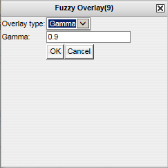
Figure 5. The Fuzzy Overlay tool. Specify the
Fuzzy Overlay type and the Gamma value (default 0.9).
Specifying the
processing extent
-
The
default processing extent of the MPM online tool is Northern Finland.
-
A
smaller rectangle for the processing extent can be drawn on the map. In case of
complex models this may be preferable to limit the processing time. The extent
rectangle can be drawn using a rectangle tool (Fig. 5) under "ModelBuilder" located on the left hand side of the MPM
online tool (Fig. 1). After selecting the tool, draw an area on the map by
clicking in one corner of the extent with the left mouse button, keeping the
mouse down and releasing it in the opposite corner of the extent.
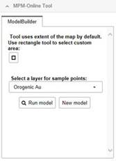
Figure 6.
The Model Builder Tool. Specify the processing extent with the rectangle tool
and the known deposits and the modelled deposit type under "Select a layer for
sample points".
-
Select
the modelled deposit type under "Select a layer for sample points". The
selection of the deposit type is only made for model validation with receiver
operating characteristics (ROC) curves and their under the area curve (AUC)
value (see FUZZY LOGIC for explanation). The data is in vector point file
format and is derived from the GTK "Mineral deposit database". Choose None if you do not want to validate your model with the ROC
tool. Naturally, the accuracy of the model is validated based on this selection
regardless of what raster inputs you have selected to the model.
Running the model
- When the geoprocessing
model in the Model Builder is ready, the processing extent is drawn on the map
and the selected deposit type is selected, the model can the executed pressing
the Run model button located in the MPM online tool (Fig. 6).
- The model is validated and the running order
is determined by performing topological sort over tool nodes in the graph. This
ensures the model is run in the correct order.
- When the model is running a "Running model..."
information window is automatically opened on top of the browser.
- All input rasters
in the model must be connected to a tool otherwise a warning will appear in the
Running model... window and model will stop running.
- When running the model the Fuzzy tool flashes
red. When the calculation is completed it turns green and plots the AUC box
next to the Fuzzy Membership or Fuzzy Overlay rectangles.
- Raster analysis output layers will appear in
the Model Builder when each step of the model is completed. A layer is
generated for Fuzzy Memberships and Fuzzy Overlay outputs for viewing.
- When the model is running the model quality
is being assessed for each input separately with ROC curves. The AUC of the ROC
curve is reported in a box after each Fuzzy membership and Fuzzy Overlay step
of the model. The ROC curve can be viewed by clicking at the AUC box appearing
next to the Fuzzy tools in the Model Builder (Fig. 7).
- AUC box will appear green when AUC >0.5
and red when AUC <0.5 (Fig. 7).
- The Running model... information window will
inform you when the model processing is completed. Press "Close" to exit the
window.
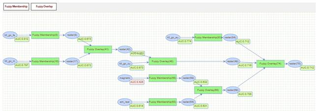
Figure 7. An example fuzzy logic model made for
orogenic gold deposits.
-
A output layers will appear under a group layer
in the ModelBuilder.
-
You
can remove the created model output layers from the ModelBuilder
and map with the button Clear geoprocessing rasters located in the ModelBuilder.
The model has to be run again in order to recreate the outputs.
-
The
rainbow colour palette (red-yellow-green-blue) with Percent Clip (1%) histogram stretching is used as
a default. Unfortunately, in the current version of the MPM online tool the
histogram stretching or classification of the colours cannot be performed by
the user.
-
When
you rerun the model again the new output layers will appear under a new group
layer. The new output layers in the Raster analysis layers have with the same layer names as in the previous
runs of the model. In case you want to compare models you must be careful and
keep your own notes how the versions of the model inputs and parameters differ
in different model runs.
-
New
model button removes the current model from the MPM online tool and opens up a
new empty Model builder window. The old model will not be saved. Do not press
the button unless you want to create a completely new model from scratch.
Visual assessment of
the model outputs
-
The
final outputs of the model can be viewed in the map and overlain by background
data from GTK and other sources.
-
The
minimum and maximum values of the outputs can be seen under Layers> layer
name>Selite.